Energy-budget evaluation in initialized decadal hindcasts
Dominik Stiller, Gregory J. Hakim, Department of Atmospheric and Climate Science, University of Washington, Seattle, WA
Poster for the Swiss Climate Summer School 2026 (Poster PDF)
Coupled models are usually evaluated on the forced response and the statistics of internal variability. Trajectories and events cannot be compared directly, because the model is not in phase with the real world. Initialization from observations synchronizes internal variability, enabling (1) event-level model evaluation and (2) estimation of predictability limits. Earth’s energy budget couples top-of-atmosphere (TOA) radiation and ocean heat content (OHC) through ocean heat uptake and the pattern-dependent radiative response, but models struggle to reproduce both. We confront the energy budget in initialized decadal hindcasts with observations: Do predictions gain the right amount of energy, and store it in the right places?
Supplemental figures
Prediction systems
We evaluate the seven CMIP6 dcppA-hindcast systems that also publish a same-resolution large ensemble and, with one exception, AMIP simulations. All scores use annual means over lead years 1–10 and starts 1960–2015.
| System | Members | Init | Strategy | Observationally constrained |
|---|---|---|---|---|
| CanESM5 | 20 | Jan | Full-field | Full coupled state (3D ocean, SST, atmosphere, sea ice); each member from its own assimilation run |
| CESM1-CAM5 | 40 | Nov | Full-field | Ocean and sea ice only, indirectly via a forced ocean–ice reconstruction; atmosphere and land not initialized. Uses CMIP5 forcings and has no AMIP simulation |
| CESM2-CAM6 | 20 | Nov | Full-field | Ocean and sea ice from a forced reconstruction; land from a JRA55-forced reconstruction; atmosphere from reanalysis |
| EC-Earth3 (i1) | 10 | Nov | Full-field | Atmosphere, land and full-depth ocean from reanalysis; sea ice only indirectly, through the nudged surface state |
| IPSL-CM6A-LR | 10 | Jan | Anomaly, surface-only | Surface ocean only (SST, Atlantic SSS); ocean interior and atmosphere free |
| MIROC6 | 10 | Nov | Mixed | Ocean temperature and salinity (anomaly), sea-ice concentration (full-field) and atmospheric states from reanalysis |
| NorCPM1 (i2) | 10 | Oct | Anomaly | Ocean (SST and hydrographic profiles) and sea ice through a coupled ensemble Kalman filter; atmosphere unconstrained |
Verification data
| Variable | Product | Period |
|---|---|---|
| Surface temperature | BEST | 1961–2024 |
| Niño 3.4 and SST | ERSSTv5 | 1961–2025 |
| TOA radiation (EEI, OLR, ASR) | CERES EBAF | 2002–2025 |
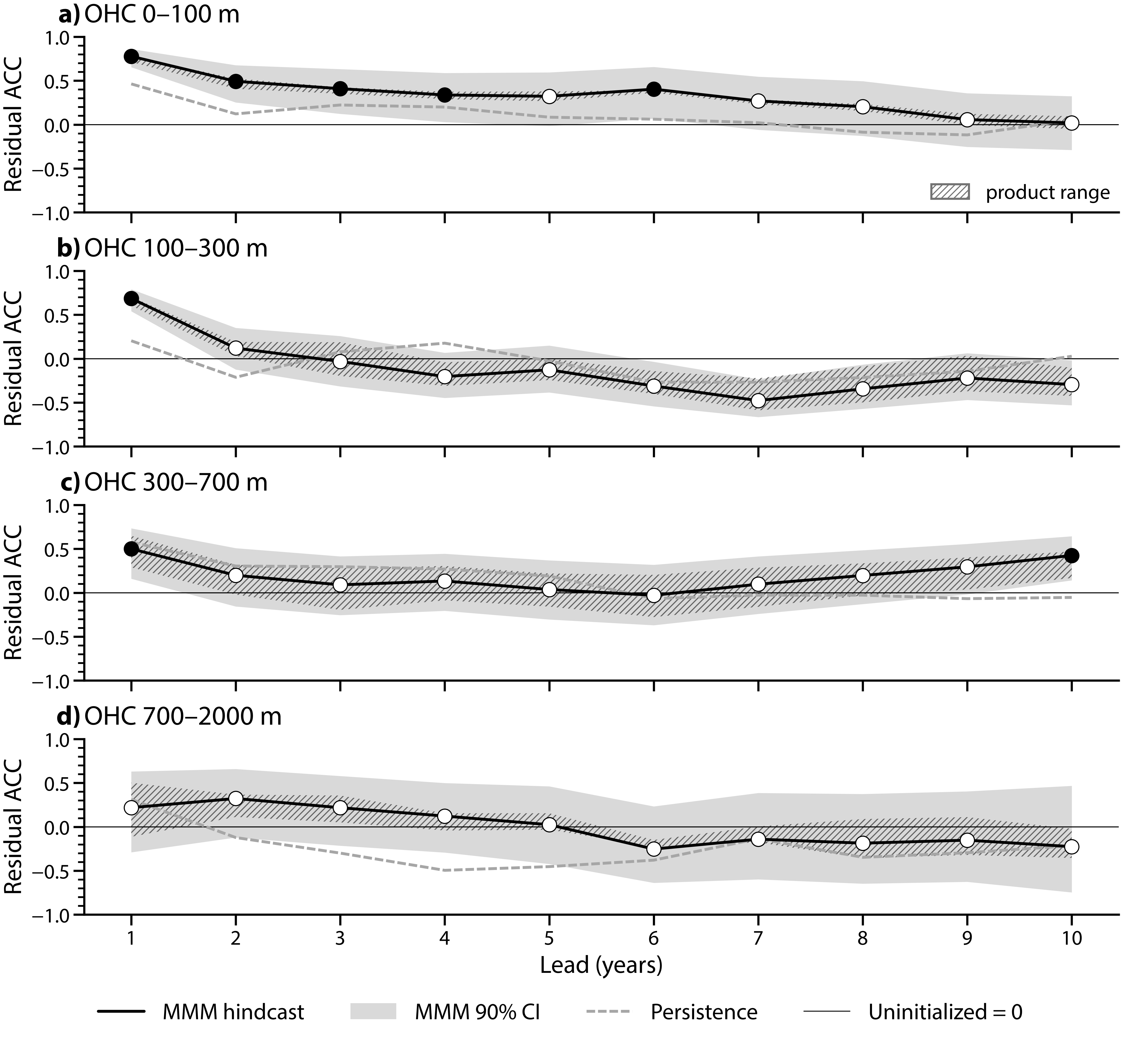
| Ocean heat content (layers) | Equal-weight mean of IAP, EN4.c14, Levitus/NCEI and Ishii/JMA with common mask | 0–700 m 1961–2024; 700–2000 m 1992–2024 (near-global coverage from 2005) |
Verification method
Alignment and sampling
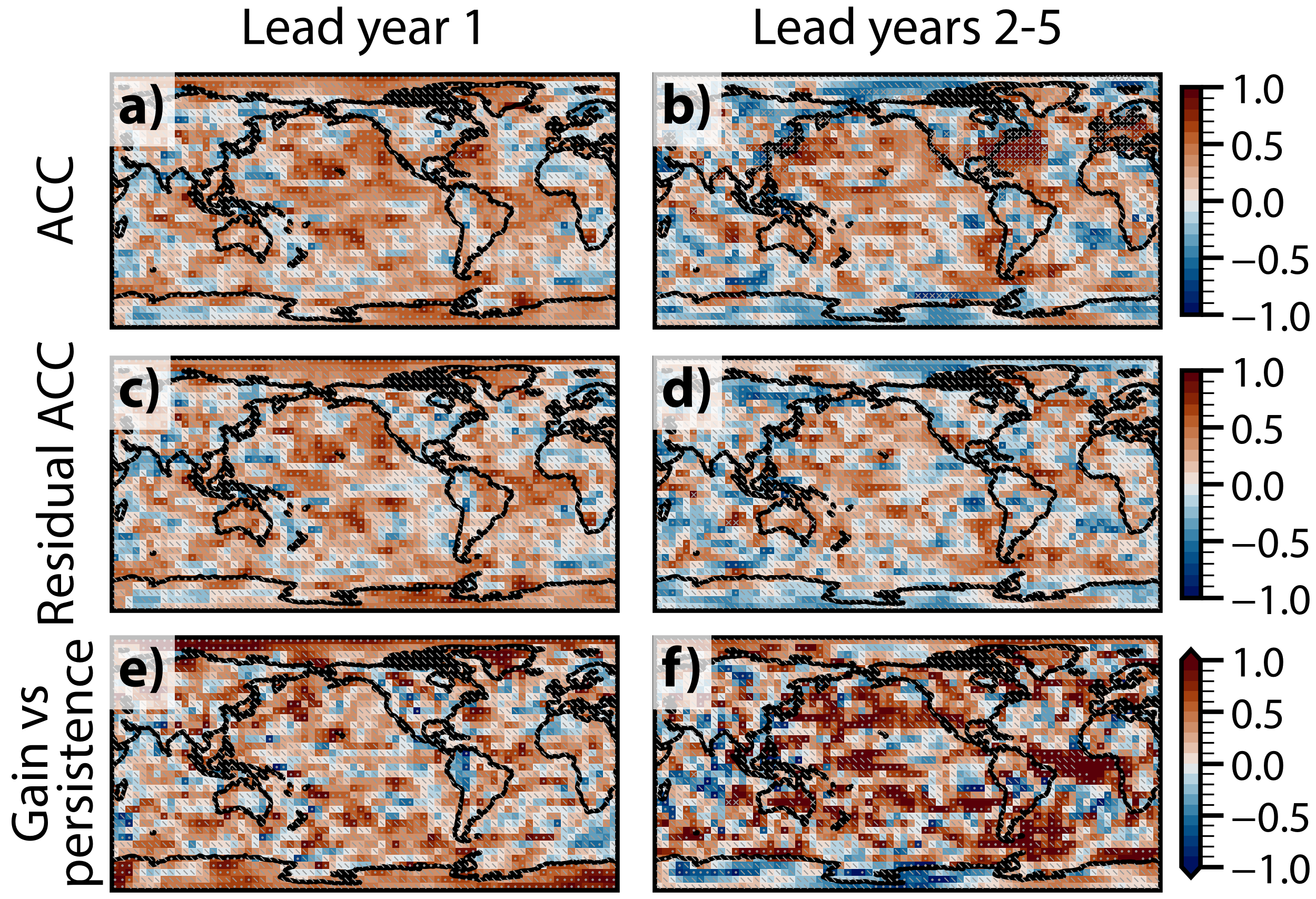
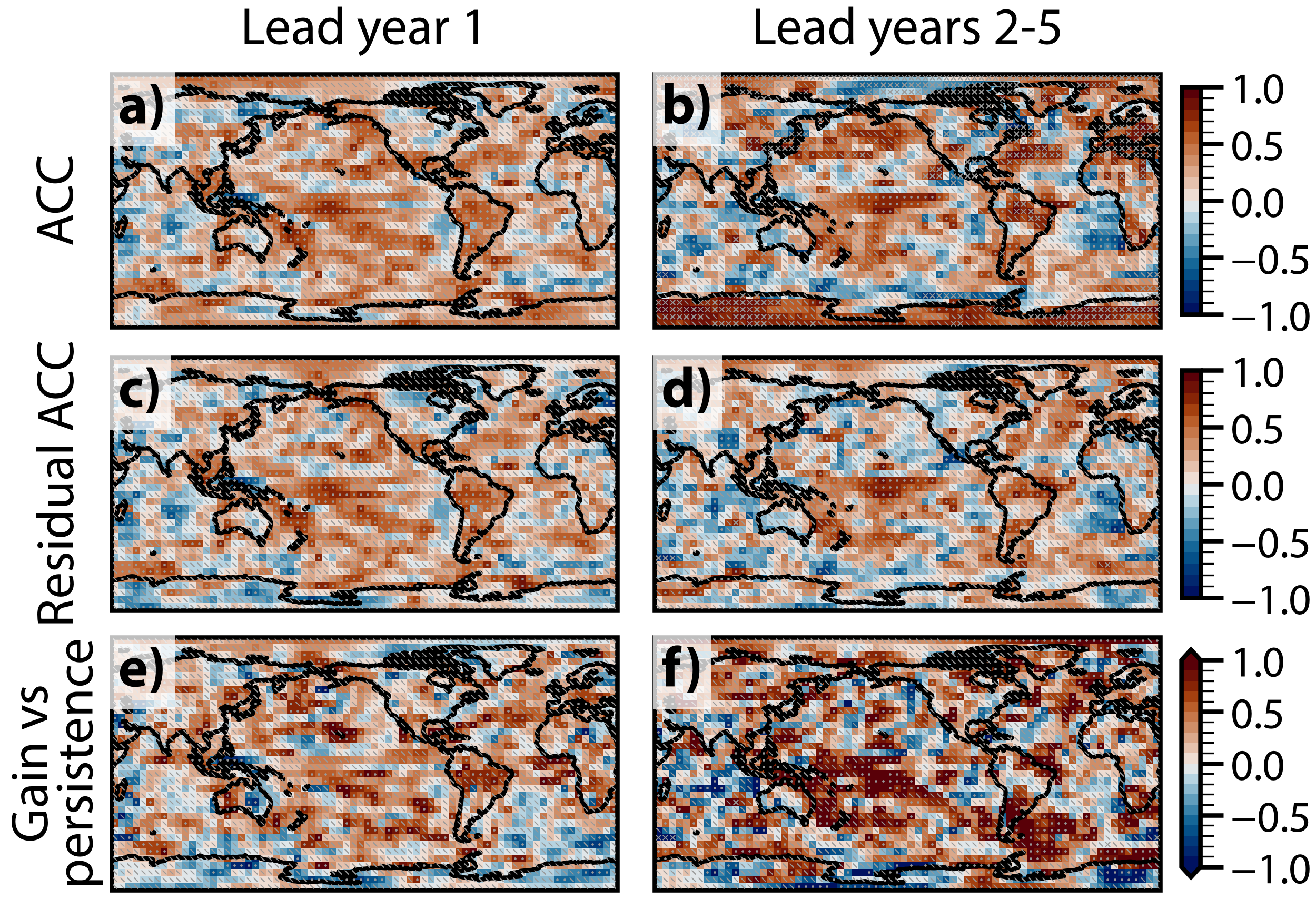
- Annual means at lead years 1–10. Maps are additionally aggregated over the multi-year windows (lead years 2–5, 6–9 and 2–9). Lead year 1 is the first calendar year fully covered by the forecast, regardless of the October, November or January start month.
- Global means of temperature and TOA flux are calculated on the native grids; ocean heat content is regridded conservatively to a 5×5° grid before any reduction, so its global means and maps share one ocean mask. All maps are on the 5×5° grid.
- Every lead is scored over the same set of starts, fixed across systems and set by the observational record: 55 starts (1960–2014) against BEST and the multi-product ocean heat content, 56 (1960–2015) against ERSST, and 15 (2001–2015) against CERES. The one exception is ocean heat content below 700 m, whose verification target begins in 1992: 24–33 starts, depending on lead.
- Re-scoring under the fixed verification window of Boer et al. (2016) moves most numbers by no more than 0.05 (except for ASR).
Bias and drift correction
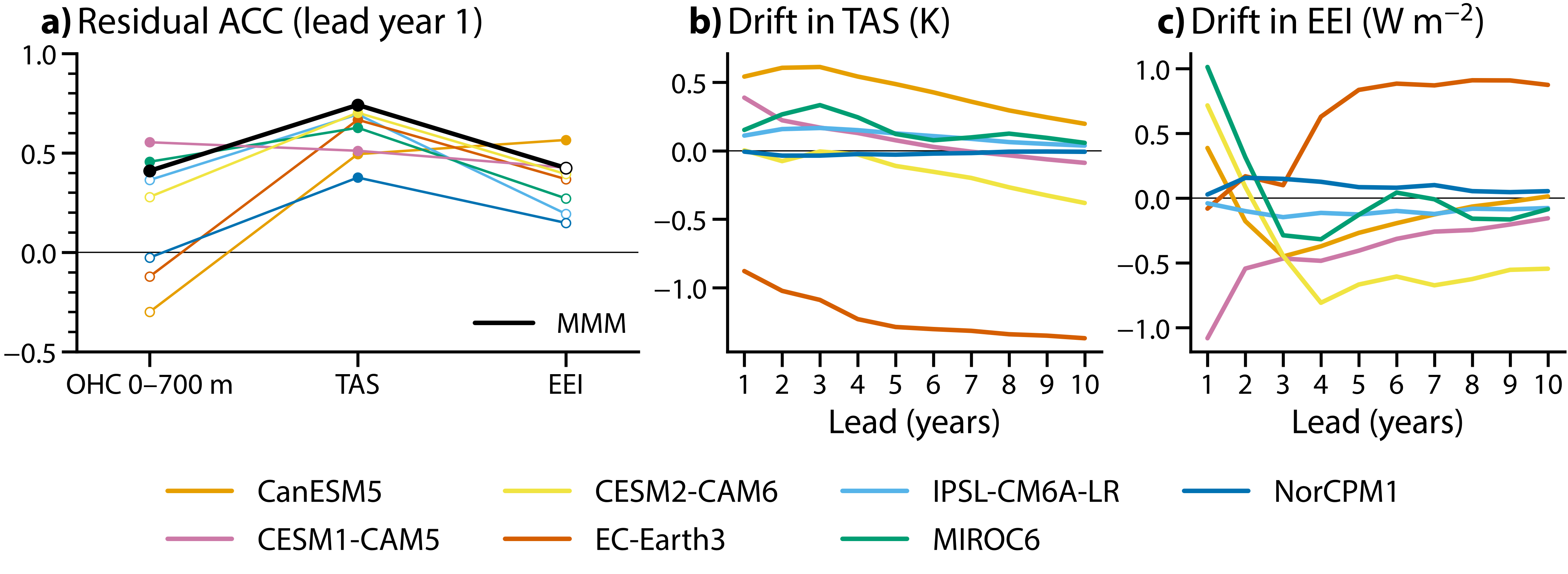
- Each series, whether hindcast, observations, or uninitialized baseline, has its own lead-dependent climatology subtracted, computed as the mean over starts at each lead. Mean bias, initialization shock and drift therefore drop out of every skill number by construction.
- Plotted full-field (non-anomaly) trajectories are treated differently: the model’s lead-dependent climatology is swapped for the observed one, so those curves keep the forced warming that the residual scores regress away.
Residual skill
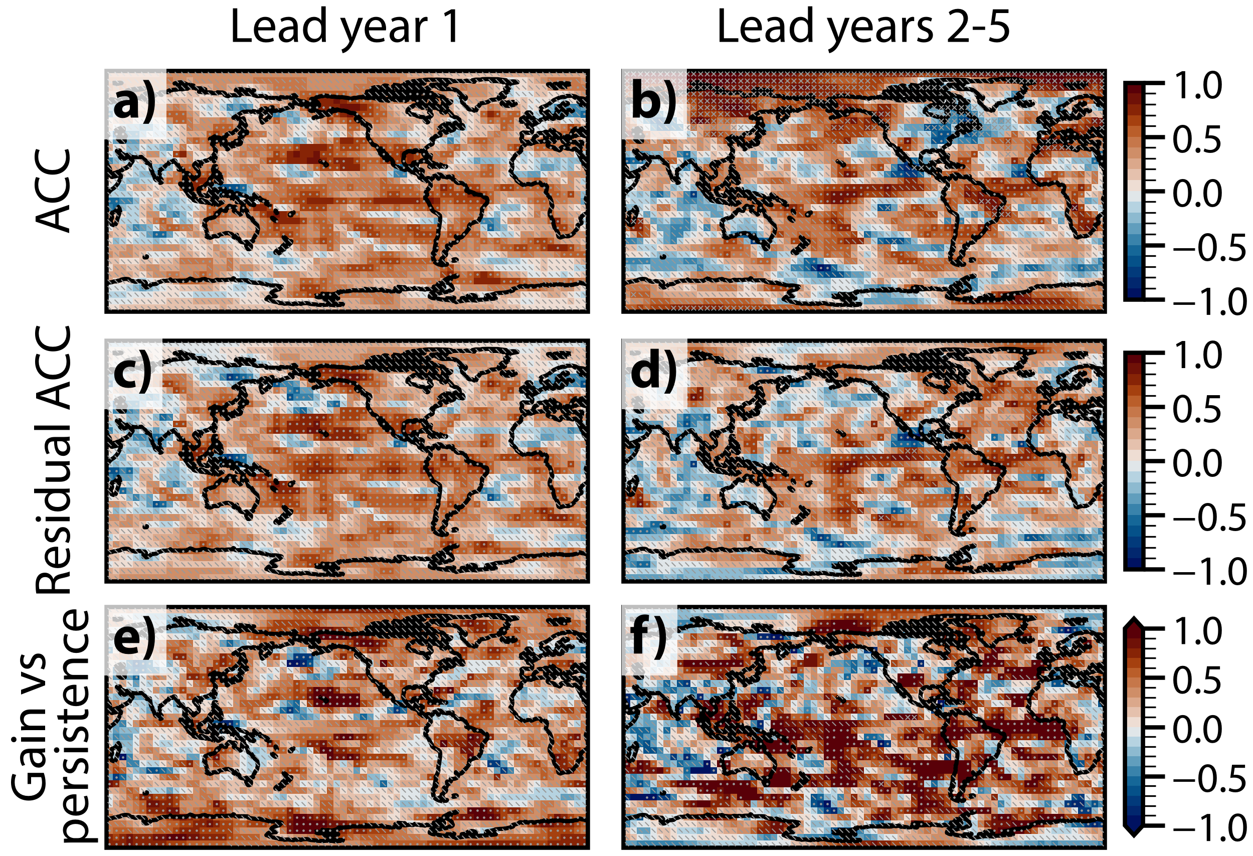
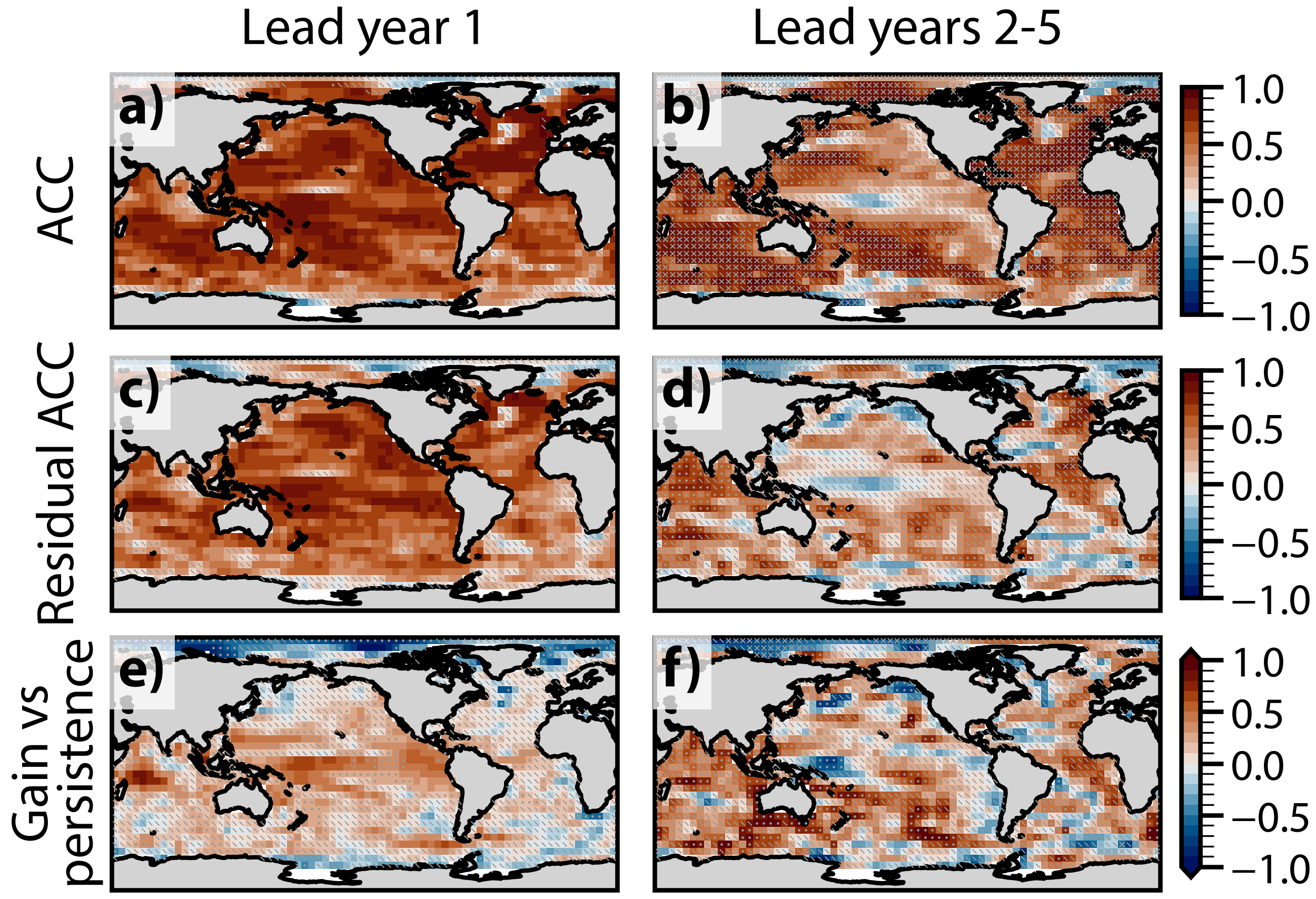
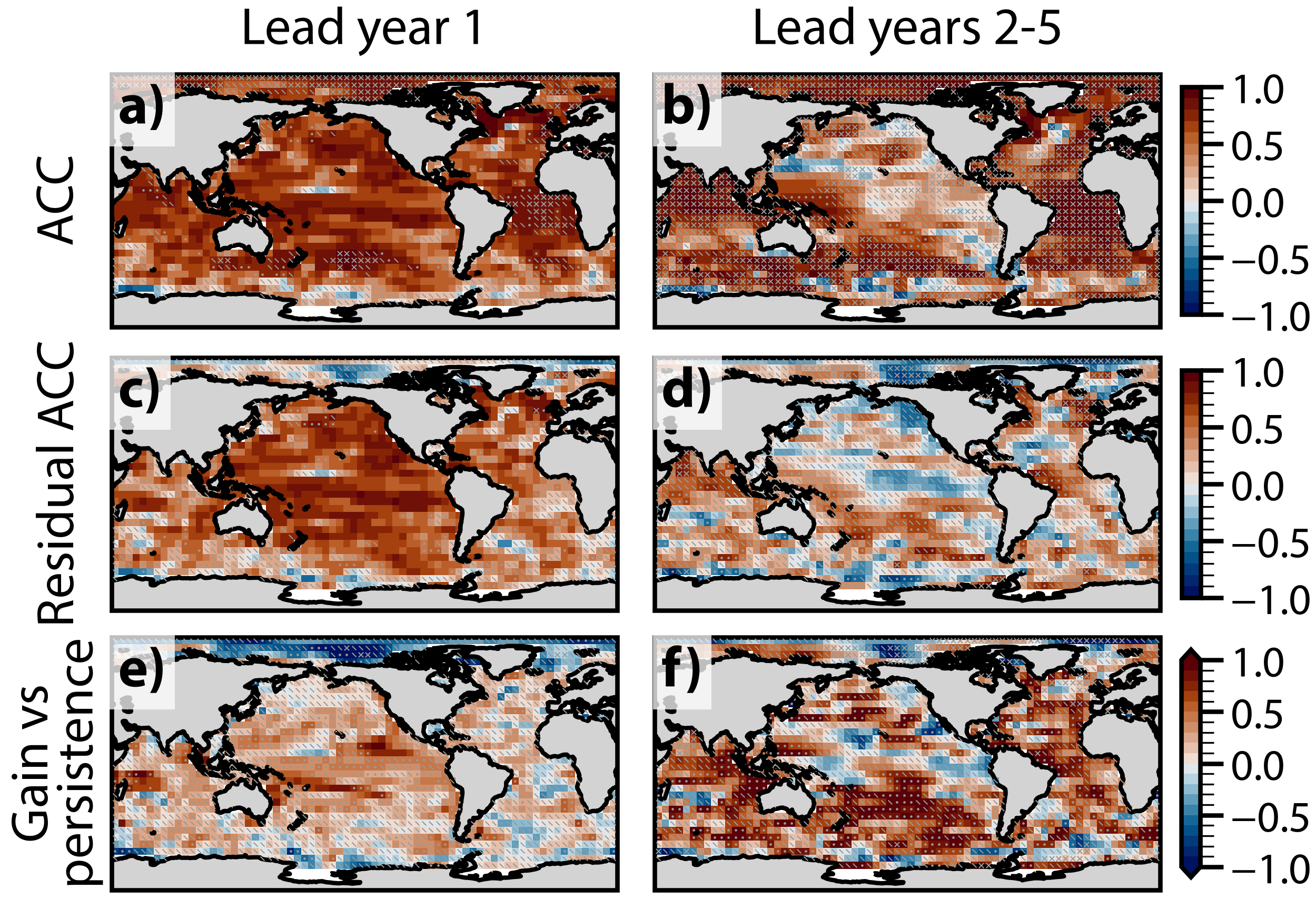
- The anomaly correlation coefficient (ACC) is the Pearson correlation between forecast and observed anomalies across starts at a given lead. It is trend saturated, reaching 0.9 to 0.98 almost everywhere, because both sides share the same forced response.
- We therefore regress an estimate of the forced response out of both sides at each lead, fitting the coefficient independently for each series. The estimate is the system’s own large ensemble mean on the forecast side, and the equal-weight multi-model mean of the seven large ensemble means on the observational side. The multi-model mean itself is scored symmetrically, with that estimate on both sides.
- The headline metric is the residual ACC, the Pearson correlation of the two residual series across starts. It is equivalently a partial correlation that controls for the forced response, following Smith et al. (2019).
- Residual figures (poster Figs. 1b and 4c) subtract the forced estimate instead of regressing it out, so plotted distances stay physical; the fitted coefficient is used only in the scores.
Significance and confidence intervals
- Uncertainty is analytic rather than bootstrapped. A block bootstrap would be biased at these sample sizes, and it rests on an arbitrary block length applied to every series alike. The analytic effective sample size is instead estimated separately for each series and lead.
- Correlations use the Fisher z transform with the effective sample size of Bretherton et al. (1999). Gains over the persistence and uninitialized baselines use the test of Steiger (1980) for dependent overlapping correlations, with the matching interval of Zou (2007). Siegert et al. (2017) recommend this test for forecast skill comparisons.
- Maps are controlled per lead with the Benjamini and Hochberg (1995) false discovery rate at 10%, following Wilks (2016).
References
Benjamini, Y., & Hochberg, Y. (1995). Controlling the false discovery rate. Journal of the Royal Statistical Society B, 57(1), 289–300. doi: 10.1111/j.2517-6161.1995.tb02031.x
Boer, G. J., Smith, D. M., Cassou, C., Doblas-Reyes, F., Danabasoglu, G., Kirtman, B., Kushnir, Y., Kimoto, M., Meehl, G. A., Msadek, R., Mueller, W. A., Taylor, K. E., Zwiers, F., Rixen, M., Ruprich-Robert, Y., & Eade, R. (2016). The Decadal Climate Prediction Project (DCPP) contribution to CMIP6. Geoscientific Model Development, 9(10), 3751–3777. doi: 10.5194/gmd-9-3751-2016
Bretherton, C. S., Widmann, M., Dymnikov, V. P., Wallace, J. M., & Bladé, I. (1999). The effective number of spatial degrees of freedom of a time-varying field. Journal of Climate, 12(7), 1990–2009. doi: 10.1175/1520-0442(1999)012<1990:tenosd>2.0.co;2
Kuhlbrodt, T., Voldoire, A., Palmer, M. D., Geoffroy, O., & Killick, R. E. (2023). Historical ocean heat uptake in two pairs of CMIP6 models: Global and regional perspectives. Journal of Climate, 36(7), 2183–2203. doi: 10.1175/JCLI-D-22-0468.1
Olonscheck, D., & Rugenstein, M. (2024). Coupled climate models systematically underestimate radiation response to surface warming. Geophysical Research Letters, 51(6), e2023GL106909. doi: 10.1029/2023GL106909
Siegert, S., Bellprat, O., Ménégoz, M., Stephenson, D. B., & Doblas-Reyes, F. J. (2017). Detecting improvements in forecast correlation skill: Statistical testing and power analysis. Monthly Weather Review, 145(2), 437–450. doi: 10.1175/MWR-D-16-0037.1
Smith, D. M., Eade, R., Scaife, A. A., Caron, L.-P., Danabasoglu, G., DelSole, T. M., Delworth, T., Doblas-Reyes, F. J., Dunstone, N. J., Hermanson, L., Kharin, V., Kimoto, M., Merryfield, W. J., Mochizuki, T., Müller, W. A., Pohlmann, H., Yeager, S., & Yang, X. (2019). Robust skill of decadal climate predictions. npj Climate and Atmospheric Science, 2(1), 13–22. doi: 10.1038/s41612-019-0071-y
Steiger, J. H. (1980). Tests for comparing elements of a correlation matrix. Psychological Bulletin, 87(2), 245–251. doi: 10.1037/0033-2909.87.2.245
Wilks, D. S. (2016). “The stippling shows statistically significant grid points”: How research results are routinely overstated and overinterpreted, and what to do about it. Bulletin of the American Meteorological Society, 97(12), 2263–2273. doi: 10.1175/BAMS-D-15-00267.1
Zou, G. Y. (2007). Toward using confidence intervals to compare correlations. Psychological Methods, 12(4), 399–413. doi: 10.1037/1082-989X.12.4.399